What this post covers
This is the eighth post in the "Digging into MariaDB's Source" series. In Part 7 we checked privileges, opened the tables and watched JOIN::prepare() tie the names in the SQL to real tables and columns. At this point the server knows what it has to read. The remaining question is how to read it: which table first, whether to use an index or scan a table from start to end. The component that makes those choices is the optimizer.
In terms of the Part 2 map, this post zooms into box ⑤ Optimization in the life of one query.
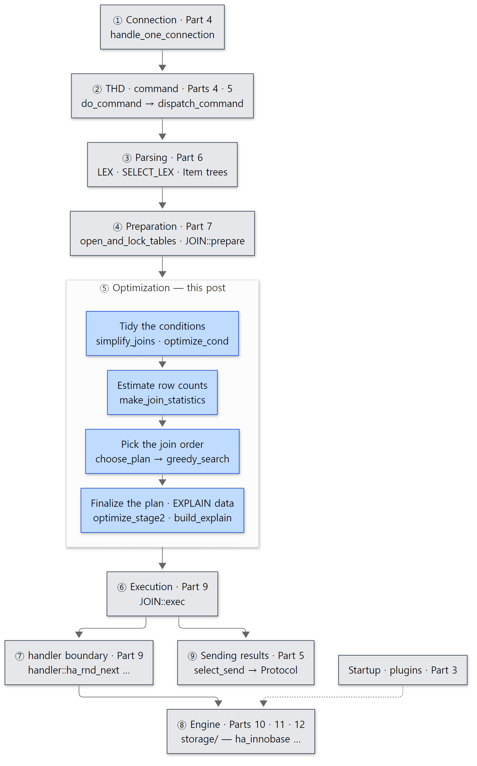 The blue boxes are what this post reads. The grey ones are covered in the posts before and after.
There are four questions to answer.
- When you type
EXPLAIN, what runs inside the server, and where do thetype,rowsandfilteredcolumns come from? - How does the optimizer know the row counts of tables it has not read yet — engine statistics, range analysis, histograms?
- With several tables, how is the join order chosen, and how are the orders it does not pick thrown away?
- What exactly is the "cost" number you see in
Last_query_cost?
| Item | Details |
|---|---|
| Target | MariaDB Server |
| Version | 13.2.0 (main, alpha) |
| Commit | c894d97781 (2026-10-19) |
| Files read most | sql/sql_select.cc, sql/opt_range.cc, sql/optimizer_costs.h·optimizer_defaults.h, sql/handler.h, sql/sql_explain.cc, sql/opt_trace.cc |
Every line number in this post refers to that commit. Part 1 explains how to get the source at the same commit and build the Docker image used for the examples.
sql/sql_select.cc is 36,086 lines and the range optimizer sql/opt_range.cc 17,993. Subquery optimization (opt_subselect.cc) alone is 7,548. This post keeps only the main thread that someone seeing the code for the first time can follow. What was left out is named, with its location, under "What this post leaves out" at the end.
Words to know first
JOIN (class JOIN, sql/sql_select.h line 1478) is the object that holds everything needed to run one SELECT block. Despite the name, a SELECT with a single table also runs through a JOIN object. Part 7's JOIN::prepare() prepares it, this post's JOIN::optimize() plans it, and Part 9's JOIN::exec() runs it. The three stages are three methods of one object.
JOIN_TAB (struct st_join_table) ties one table in the join to "how that table will be read". Think of one line of EXPLAIN as one JOIN_TAB. EXPLAIN's type column (ALL, ref, eq_ref, const …) is the enum join_type value in JOIN_TAB::type turned into text (join_type_str[], sql/sql_select.cc line 122).
POSITION (sql/sql_select.h line 1248) is one candidate: "put this table in slot N of the join order, read it this way". It holds the rows to read (records_read), the rows left after the WHERE clause (records_out) and the cost (read_time). JOIN::positions[] is the order being examined right now; JOIN::best_positions[] is the best order found so far.
KEYUSE is one equality such as t.col = something that an index can be used to look up. Collecting them from WHERE and ON up front (update_ref_and_keys()) means the optimizer can later tell at once "what must already have been read before this table can be looked up through this index".
SEL_TREE and SEL_ARG are the containers the range optimizer uses to turn WHERE into "intervals on an index". country = 'KR' becomes the interval [KR, KR] on idx_country. We look at them in section 4.
Cost is the score the optimizer gives plans so it can compare them. You can see it in the session status variable Last_query_cost. In this commit the cost has a fixed unit — 1 is one millisecond (section 5).
A const table is a table that is known to produce at most one row. The optimizer reads such a table while it is still planning and treats its values as constants (section 3).
1. JOIN::optimize() — the main thread
We saw the path of one SELECT in Part 2. mysql_select() calls JOIN::prepare() (line 5432) → JOIN::optimize() (line 5447) → JOIN::exec() (line 5461) in turn.
EXPLAIN takes the same path. execute_sqlcom_select() looks at lex->describe (the flag set for EXPLAIN) and calls mysql_explain_union(), which ends up calling the same mysql_select() (we confirm this in the backtrace of Example 4 below). So the plan EXPLAIN shows is the plan made by the same functions that run the real query. The only difference is that instead of reading rows inside JOIN::exec(), it prints the plan and returns (the SELECT_DESCRIBE branch of exec_inner(), lines 5114–5120).
JOIN::optimize() itself is short.
int JOIN::optimize()
{
  int res= 0;
  if (select_lex->pushdown_select)
  // ... (an engine takes the whole SELECT (select_handler) — omitted)
  else
  {
    // ...
    if (optimization_state != JOIN::NOT_OPTIMIZED)
      return FALSE;
    optimization_state= JOIN::OPTIMIZATION_IN_PROGRESS;
    res= optimize_inner();
  }
  if (!with_two_phase_optimization)
  {
    if (!res && have_query_plan != QEP_DELETED)
      res= build_explain();
    optimization_state= JOIN::OPTIMIZATION_DONE;
  }

  // ...
  if (select_lex->select_number == 1)
    thd->status_var.last_query_cost= best_read;
  return res;
}
sql/sql_select.cc lines 2004–2048
Three things can be read here.
- It runs only once. If
optimization_stateis notNOT_OPTIMIZED, it returns right away. The sameJOINcan be called more than once, for example for a subquery, so the door is guarded. - The real work is in
optimize_inner(). When it finishes,build_explain()makes a separate copy of the data EXPLAIN will print (section 8). - This is where
Last_query_costcomes from. Thebest_read— the cost of the chosen plan — of the outermostSELECT(select_number == 1) is written to the session status variable.
optimize_inner() is a function of about 600 lines (lines 2230–2809). Listing just the big pieces in order:
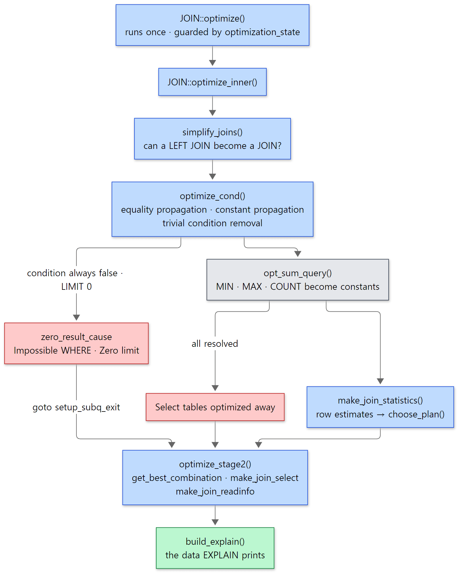 The red boxes are shortcuts where the answer is settled without reading any table.
| Step | What it does | Where |
|---|---|---|
| 1 | Turn outer joins into inner joins where possible simplify_joins() |
line 2378 |
| 2 | Tidy up WHERE optimize_cond() |
line 2494 |
| 3 | Stop here if the condition is always false (Impossible WHERE) |
lines 2619–2640 |
| 4 | Partition pruning prune_partitions() |
lines 2643–2654 |
| 5 | Get MIN()·MAX()·COUNT(*) straight from index ends or statistics opt_sum_query() |
lines 2662–2739 |
| 6 | Estimate row counts and pick the join order make_join_statistics() |
line 2779 |
| 7 | Build the JOIN_TABs in the chosen order and hand each table its conditions optimize_stage2() |
line 2805 |
Inside step 7, optimize_stage2(), get_best_combination() (line 2839) builds the JOIN_TAB array in best_positions[] order, make_join_select() (line 3091) splits WHERE and attaches each piece to a table ("check this condition when reading this table"), and make_join_readinfo() (line 3385) picks a read function for each table. We see those read functions actually being called in Part 9.
Example 1: EXPLAIN and Last_query_cost
The examples use a tiny shop: 1,000 customers and 20,000 orders, of which only about 1% have status = 'cancelled'. Every example in this post uses the same setup.sql.
-- Written for this post (not part of MariaDB's source)
-- 1,000 customers and 20,000 orders. Only about 1% of the orders are 'cancelled'.
CREATE DATABASE shop;
USE shop;
CREATE TABLE customers (
  id INT PRIMARY KEY,
  name VARCHAR(30),
  country CHAR(2),
  KEY idx_country (country)
) ENGINE=InnoDB;
CREATE TABLE orders (
  id INT PRIMARY KEY,
  customer_id INT NOT NULL,
  status VARCHAR(10) NOT NULL,
  amount INT NOT NULL
) ENGINE=InnoDB;
-- seq_1_to_N is a virtual table provided by the SEQUENCE engine
INSERT INTO customers
  SELECT seq, CONCAT('customer-', seq),
         ELT(1 + seq % 10, 'KR','US','JP','DE','FR','GB','CN','IN','BR','CA')
  FROM seq_1_to_1000;
INSERT INTO orders
  SELECT seq, 1 + seq % 1000, IF(seq % 97 = 0, 'cancelled', 'done'), seq % 500
  FROM seq_1_to_20000;
-- refresh the engine statistics (InnoDB's row count and index cardinality)
ANALYZE TABLE customers, orders;
[Example ex/u08-explain-basics/setup.sql — the same file is in all four example folders]
This example and the others in this post were run in a Docker container (Ubuntu 24.04) with MariaDB 13.2.0 (13.2.0-MariaDB-debug), a Debug build of the reference commit (c894d97781) as is. The first example is a join that finds "cancelled orders of Korean customers". There is no index on orders.customer_id yet.
EXPLAIN SELECT c.name, o.amount
  FROM customers c JOIN orders o ON o.customer_id = c.id
  WHERE c.country = 'KR' AND o.status = 'cancelled';
-- JOIN::optimize() leaves best_read here
SHOW SESSION STATUS LIKE 'Last_query_cost';
+------+-------------+-------+--------+---------------------+---------+---------+--------------------+-------+-------------+
 id   | select_type | table | type   | possible_keys       | key     | key_len | ref                | rows  | Extra       |
+------+-------------+-------+--------+---------------------+---------+---------+--------------------+-------+-------------+
    1 | SIMPLE      | o     | ALL    | NULL                | NULL    | NULL    | NULL               | 19982 | Using where |
    1 | SIMPLE      | c     | eq_ref | PRIMARY,idx_country | PRIMARY | 4       | shop.o.customer_id | 1     | Using where |
+------+-------------+-------+--------+---------------------+---------+---------+--------------------+-------+-------------+
+-----------------+-----------+
 Variable_name   | Value     |
+-----------------+-----------+
 Last_query_cost | 21.226778 |
+-----------------+-----------+
The SQL lists customers first, but the optimizer scans orders first (ALL) and looks up customers once per order through the primary key (eq_ref). Without an index on orders.customer_id, orders has to be scanned in full whichever order is chosen, so it computed that scanning orders first and looking up customers by primary key is cheaper (we follow the computation in sections 5 and 6). The 19982 in rows is InnoDB's estimate of the row count (the real number is 20,000 — section 3).
EXPLAIN FORMAT=JSON on the same plan shows the cost of each table (output 6 of the same example, with a few key-related lines of c cut to ...).
{
  "query_block": {
    "select_id": 1,
    "cost": 21.22677768,
    "nested_loop": [
      {
        "table": {
          "table_name": "o",
          "access_type": "ALL",
          "loops": 1,
          "rows": 19982,
          "cost": 3.3499816,
          "filtered": 100,
          "attached_condition": "o.`status` = 'cancelled'"
        }
      },
      {
        "table": {
          "table_name": "c",
          "access_type": "eq_ref",
          ...
          "loops": 19982,
          "rows": 1,
          "cost": 17.87679608,
          "filtered": 10,
          "attached_condition": "c.country = 'KR'"
        }
      }
    ]
  }
}
3.35 to scan o, 17.88 to look up c 19,982 times (loops); together they are the query_block's 21.23, which is Last_query_cost. Keep in mind that most of the cost comes from "the number of lookups" — that is exactly why the plan changes in section 7. Also note o's "filtered": 100: the optimizer believes status = 'cancelled' filters out nothing. We come back to that in section 7 too.
That each table carries its own "attached_condition" is the result of make_join_select() mentioned above. c.country = 'KR' is checked when reading c, and o.status = 'cancelled' when reading o.
Easy to get wrong: EXPLAIN's rows is not "the number of result rows"
rows is the estimated number of rows read when the table is read once with that access method. It repeats for every row of the tables before it, so the amount actually read is that times the row count of the earlier tables (loops in the JSON). It is also the number before WHERE filtering; the fraction left after filtering is shown separately in filtered. The source makes this explicit where best_access_path() records its choice: "We use 'records' instead of 'records_after_filter' here as we want to have EXPLAIN print the number of rows found by the key access" (lines 9786–9790).
2. Tidying the conditions — optimize_cond() and simplify_joins()
Before counting rows, the optimizer tidies up WHERE: into a shape that is easier to work with when the meaning is the same, and with pieces that are always true or always false removed. optimize_cond() does this.
    conds= build_equal_items(join, conds, NULL, join_list,
                             ignore_on_conds, cond_equal,
                             MY_TEST(flags & OPT_LINK_EQUAL_FIELDS));
    // ... (records equality_propagation in the trace)
    /* change field = field to field = const for each found field = const */
    propagate_cond_constants(thd, (I_List<COND_CMP> *) 0, conds, conds);
    /*
      Remove all instances of item == item
      Remove all and-levels where CONST item != CONST item
    */
    // ... (records constant_propagation in the trace)
    conds= conds->remove_eq_conds(thd, cond_value, true);
    if (conds && conds->type() == Item::COND_ITEM &&
        ((Item_cond*) conds)->functype() == Item_func::COND_AND_FUNC)
      *cond_equal= &((Item_cond_and*) conds)->m_cond_equal;
sql/sql_select.cc lines 21080–21110
There are three steps, and at the end of each one the name is written to optimizer_trace (you can see them exactly as is in Example 3 of section 6).
- Equality propagation (
build_equal_items()). Columns and constants linked by equalities, likeo.customer_id = c.id AND c.id = 5, are bundled into a singleItem_equal. The trace prints it asmultiple equal(o.customer_id, c.id). Once bundled, the server knows "o.customer_idis also 5" without writing it down separately. AnItemis a node of the condition tree we saw in Part 6. - Constant propagation (
propagate_cond_constants()). Once it knowscolumn = constant, it puts the constant wherever else that column appears. - Trivial condition removal (
remove_eq_conds()). Pieces that are always true, like1 = 1, are removed; if the whole thing is always false, it reportsCOND_FALSEthroughcond_value.
When COND_FALSE comes back, optimize_inner() ends without reading a single table (lines 2619–2640). It writes "Impossible WHERE" into zero_result_cause, or "Zero limit" for LIMIT 0, and that text appears as is in EXPLAIN's Extra. In the same function, when opt_sum_query() resolves MIN()·MAX()·COUNT(*) without any table, "Select tables optimized away" is written (line 2710).
Example 1 (continued): queries answered before any table is read
EXPLAIN SELECT * FROM customers WHERE id = 5 AND id = 6;
EXPLAIN SELECT MIN(id), MAX(id) FROM orders;
EXPLAIN SELECT * FROM customers WHERE country = 'KR' LIMIT 0;
+------+-------------+-------+------+---------------+------+---------+------+------+------------------+
 id   | select_type | table | type | possible_keys | key  | key_len | ref  | rows | Extra            |
+------+-------------+-------+------+---------------+------+---------+------+------+------------------+
    1 | SIMPLE      | NULL  | NULL | NULL          | NULL | NULL    | NULL | NULL | Impossible WHERE |
+------+-------------+-------+------+---------------+------+---------+------+------+------------------+
+------+-------------+-------+------+---------------+------+---------+------+------+------------------------------+
 id   | select_type | table | type | possible_keys | key  | key_len | ref  | rows | Extra                        |
+------+-------------+-------+------+---------------+------+---------+------+------+------------------------------+
    1 | SIMPLE      | NULL  | NULL | NULL          | NULL | NULL    | NULL | NULL | Select tables optimized away |
+------+-------------+-------+------+---------------+------+---------+------+------+------------------------------+
+------+-------------+-------+------+---------------+------+---------+------+------+------------+
 id   | select_type | table | type | possible_keys | key  | key_len | ref  | rows | Extra      |
+------+-------------+-------+------+---------------+------+---------+------+------+------------+
    1 | SIMPLE      | NULL  | NULL | NULL          | NULL | NULL    | NULL | NULL | Zero limit |
+------+-------------+-------+------+---------------+------+---------+------+------+------------+
id = 5 AND id = 6 becomes, during equality propagation, an Item_equal in which id has to be both 5 and 6, so it is judged always false. table is NULL — there is no table in the plan at all. MIN(id)·MAX(id) only need one look at each end of the primary-key B-tree, so the optimizer works out the values themselves during optimization.
Where a LEFT JOIN becomes a JOIN
simplify_joins() checks whether an outer join can be turned into an inner join. The heart of it is this condition.
    if (!(table->outer_join & (JOIN_TYPE_LEFT | JOIN_TYPE_RIGHT)) ||
        (used_tables & not_null_tables))
    {
      /*
        For some of the inner tables there are conjunctive predicates
        that reject nulls => the outer join can be replaced by an inner join.
      */
      if (table->outer_join && !table->embedding && table->table)
        table->table->maybe_null= FALSE;
      table->outer_join= 0;
sql/sql_select.cc lines 20248–20257
not_null_tables is "the tables that must not be NULL for this WHERE to be true". With LEFT JOIN orders o … WHERE o.status = 'cancelled', a row where o found no match and was filled with NULLs can never make o.status = 'cancelled' true, so it is thrown away anyway. Then there is no reason to keep the LEFT JOIN. outer_join= 0 makes it an inner join, and right below the ON condition is merged into WHERE with and_conds() (lines 20273–20287).
EXPLAIN EXTENDED SELECT c.name, o.amount
  FROM customers c LEFT JOIN orders o ON o.customer_id = c.id
  WHERE o.status = 'cancelled';
SHOW WARNINGS;
+------+-------------+-------+--------+---------------+---------+---------+--------------------+-------+----------+-------------+
 id   | select_type | table | type   | possible_keys | key     | key_len | ref                | rows  | filtered | Extra       |
+------+-------------+-------+--------+---------------+---------+---------+--------------------+-------+----------+-------------+
    1 | SIMPLE      | o     | ALL    | NULL          | NULL    | NULL    | NULL               | 19982 |   100.00 | Using where |
    1 | SIMPLE      | c     | eq_ref | PRIMARY       | PRIMARY | 4       | shop.o.customer_id | 1     |   100.00 |             |
+------+-------------+-------+--------+---------------+---------+---------+--------------------+-------+----------+-------------+
+-------+------+----------------------------------------------------------------------------------------------------------------------------------------------------------------------------------------------------------------+
 Level | Code | Message                                                                                                                                                                                                        |
+-------+------+----------------------------------------------------------------------------------------------------------------------------------------------------------------------------------------------------------------+
 Note  | 1003 | select `shop`.`c`.`name` AS `name`,`shop`.`o`.`amount` AS `amount` from `shop`.`customers` `c` join `shop`.`orders` `o` where `shop`.`c`.`id` = `shop`.`o`.`customer_id` and `shop`.`o`.`status` = 'cancelled' |
+-------+------+----------------------------------------------------------------------------------------------------------------------------------------------------------------------------------------------------------------+
The Note from SHOW WARNINGS is the query printed back after the optimizer has tidied it (Part 6). left join became join, and the ON condition moved into where. And in the plan, o came first. Under a LEFT JOIN, o hangs off c and cannot be read before c (dep_tables). Turning it into an inner join lifted that restriction, so the optimizer could pick the same order as in the first example of section 1.
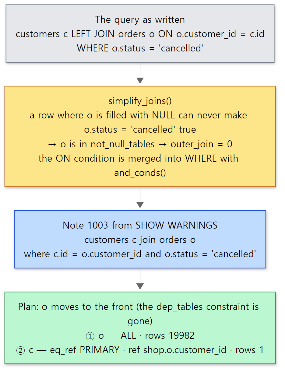 A single condition on the right-hand table written in WHERE turns the LEFT JOIN into a JOIN, and that in turn changes the join order. The query and the plan are the actual output of the example above.
Easy to get wrong: a right-table condition in WHERE
This is a common mistake in application code. You write a LEFT JOIN "so that customers with no cancelled orders also show up", but put the filter in WHERE, and the server quietly turns it into an inner join as above. The result is not wrong — that is simply what the SQL means. To keep customers without a match, the condition has to go into ON, as in ON o.customer_id = c.id AND o.status = 'cancelled'. Checking with EXPLAIN EXTENDED + SHOW WARNINGS whether left join survived is a useful habit.
3. Counting rows — make_join_statistics()
Once the conditions are tidy, make_join_statistics() (about 800 lines from line 5670) estimates "how many rows will be read" for each table and, at the end, calls the join-order search (choose_plan()).
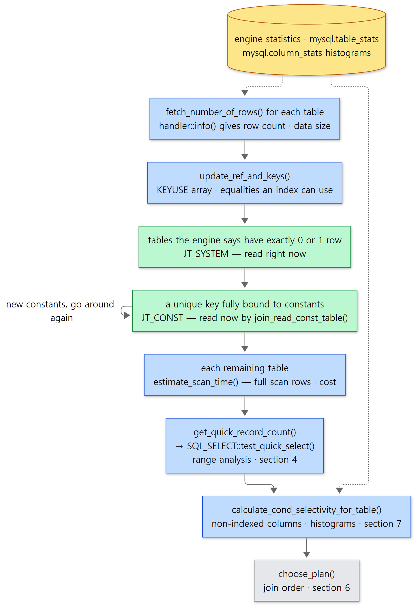 The two green boxes are where tables are actually read while the plan is still being made.
Asking the engine for the row count
The first step is to ask the engine how big each table is. For an ordinary table, TABLE_LIST::fetch_number_of_rows() calls handler::info().
  if (is_materialized_derived() && !fill_me)
  {
    table->file->stats.records= get_unit()->result->est_records;
    set_if_bigger(table->file->stats.records, 2);
    table->used_stat_records= table->file->stats.records;
  }
  else
    error= table->file->info(HA_STATUS_VARIABLE | HA_STATUS_NO_LOCK);
  return error;
sql/table.cc lines 10489–10497
handler::info() is a virtual function each engine implements (the handler from Part 2). HA_STATUS_VARIABLE asks it to fill in "values that change often, like the row count and data size", and InnoDB fills stats.records from its own statistics in ha_innobase::info() (ha_innodb.cc line 15508). TABLE_ROWS in information_schema.TABLES shows the same value (output 0 of Example 2 shows 19982 for orders). InnoDB's row count is an estimate derived from its statistics, so it differs a little from the real 20,000.
Const tables — read while the plan is being made
Next comes finding const tables. If every column of a unique index (the primary key or a UNIQUE key) is bound by equalities to constants, the result has at most one row. The optimizer marks the table JT_CONST and reads it on the spot.
              if (base_const_ref == base_eq_part &&
                  !has_expensive_keyparts &&
                  !((outer_join & table->map) &&
                    (*s->on_expr_ref)->is_expensive()))
              {                                 // Found everything for ref.
                int tmp;
                ref_changed = 1;
                s->type= JT_CONST;
                join->const_table_map|=table->map;
                set_position(join,const_count++,s,start_keyuse);
                // ... (create_ref_for_key() — prepares the key value to look up)
                if ((tmp=join_read_const_table(join->thd, s,
                                               join->positions+const_count-1)))
                {
                  if (tmp > 0)
                    goto error;                 // Fatal error
                }
                else
                  found_const_table_map|= table->map;
sql/sql_select.cc lines 6070–6091
join_read_const_table() is the function that actually reads one row from the engine (line 25986). The row's values are used as constants from then on, so conditions on other tables connected to this one can become "column = constant" in turn. That is why finding const tables repeats until no new const table appears (the do { … } while (ref_changed) on lines 5927–6101). The comment on JT_CONST in enum join_type says the same: the optimizer "fetches the row once during optimization with a single exact key lookup" (sql/sql_select.h lines 223–236).
Example 1 (continued): EXPLAIN alone read from the engine
FLUSH STATUS;
EXPLAIN SELECT * FROM customers WHERE id = 5;
-- only EXPLAIN, yet the engine was read once
SHOW SESSION STATUS LIKE 'Handler_read_key';
+------+-------------+-----------+-------+---------------+---------+---------+-------+------+-------+
 id   | select_type | table     | type  | possible_keys | key     | key_len | ref   | rows | Extra |
+------+-------------+-----------+-------+---------------+---------+---------+-------+------+-------+
    1 | SIMPLE      | customers | const | PRIMARY       | PRIMARY | 4       | const | 1    |       |
+------+-------------+-----------+-------+---------------+---------+---------+-------+------+-------+
+------------------+-------+
 Variable_name    | Value |
+------------------+-------+
 Handler_read_key | 1     |
+------------------+-------+
Handler_read_key is a status variable that goes up by one each time a handler finds a row through an index (Part 9). After resetting it to 0 with FLUSH STATUS, we ran only EXPLAIN, and it became 1. The const table was read not during execution but already during optimization.
Easy to get wrong: you rarely see "system" with InnoDB
EXPLAIN's type also has system, which is stronger than const (a table with only 0 or 1 rows). But for an ordinary table it is chosen only when the engine reports an exact row count — the condition is table->file->stats.records <= 1 && (ha_table_flags() & HA_STATS_RECORDS_IS_EXACT) (lines 5828–5832; the same condition also holds a few rare exceptions, such as a table whose partitions were all pruned away). MyISAM (ha_myisam.cc line 731) and Aria (ha_maria.cc line 1003) have that flag; InnoDB does not. In output 2b of Example 1, EXPLAIN on a one-row table that differs only in its engine splits exactly that way.
|    1 | SIMPLE      | one_innodb | ALL  | NULL          | NULL | NULL    | NULL | 1    |       |
    1 | SIMPLE      | one_myisam | system | NULL          | NULL | NULL    | NULL | 1    |       |
(Only the data lines of the two EXPLAIN tables are copied here.)
For each remaining table: full scan, ranges, selectivity
For each table that is not const, three things are worked out.
      if ((!s->const_keys.is_clear_all() ||                            // (1)
           !bitmap_is_clear_all(&s->table->cond_set) ||                // (2)
           thd->variables.optimizer_use_condition_selectivity >= 5) && // (3)
          !s->table->is_filled_at_execution() &&                       // (4)
          !(s->table->pos_in_table_list->derived &&                    // (5)
            s->table->pos_in_table_list->is_materialized_derived()))   // (5)
      // ... (builds an SQL_SELECT from WHERE)
          if (get_quick_record_count(join->thd, select, s->table,
                                     &s->const_keys, join->row_limit, &records))
sql/sql_select.cc lines 6243–6266
- The rows and cost of a full scan —
s->estimate_scan_time()just before this excerpt (line 6216, defined on line 17123). Whatever the plan, "read from start to end" is always possible, so this is the baseline. - Range analysis — if WHERE has a condition on an indexed column (
const_keys),get_quick_record_count()→SQL_SELECT::test_quick_select()works out "how many rows if we narrow it with the index". That is the topic of section 4. - Condition selectivity — if
optimizer_use_condition_selectivityis greater than 1,calculate_cond_selectivity_for_table()(line 6294) estimates "what percentage remains" even for conditions on non-indexed columns. This is where histograms are used (section 7).
The KEYUSE array built by update_ref_and_keys() (line 7756) is only used for finding const tables at this stage; its real use is the join-order search that follows. "If the earlier table has been read, this index can be used to look rows up" becomes the ref·eq_ref candidates.
4. The range optimizer — turning WHERE into intervals on an index
SQL_SELECT::test_quick_select() in sql/opt_range.cc works out, for one table, "how cheap is it to read intervals on an index?" The first thing it does is set the bar to beat.
  if (head->force_index || force_quick_range)
  {
    DEBUG_SYNC(thd, "in_forced_range_optimize");
    read_time= DBL_MAX;
  }
  else
  {
    read_time= file->cost(file->ha_scan_and_compare_time(records));
    if (limit < records)
      notnull_cond= nullptr;
  }
sql/opt_range.cc lines 2760–2770
The full scan cost becomes read_time, and only range plans that come in under it are accepted. With FORCE INDEX, the bar is set to infinity (DBL_MAX) so that any range plan wins. After setting the bar, it turns WHERE into intervals.
if (cond)
tree= cond->get_mm_tree(¶m, &cond);
if (notnull_cond_tree)
tree= tree_and(¶m, tree, notnull_cond_tree);
// ... (trace of the SEL_ARG count limit, etc.)
if (tree->type == SEL_TREE::IMPOSSIBLE)
{
records=0L;
returnval= IMPOSSIBLE_RANGE;
sql/opt_range.cc lines 2979–2996
get_mm_tree() is a virtual function of the Item tree. It is implemented separately for each kind of node, and it builds up a SEL_TREE as it walks down the tree. An AND node combines its children's results with tree_and().
SEL_TREE *Item_cond_and::get_mm_tree(RANGE_OPT_PARAM *param, Item **cond_ptr)
{
  DBUG_ENTER("Item_cond_and::get_mm_tree");
  SEL_TREE *tree= NULL;
  List_iterator<Item> li(*argument_list());
  Item *item;
  while ((item= li++))
  {
    SEL_TREE *new_tree= li.ref()[0]->get_mm_tree(param,li.ref());
    if (param->statement_should_be_aborted())
      DBUG_RETURN(NULL);
    tree= tree_and(param, tree, new_tree);
    if (tree && tree->type == SEL_TREE::IMPOSSIBLE)
    {
      // ... (if IMPOSSIBLE, return it as is)
      break;
    }
  }
  DBUG_RETURN(tree);
sql/opt_range.cc lines 8909–8931
An OR node (Item_cond::get_mm_tree(), line 8935) merges them with tree_or(). At the bottom, a comparison like country = 'KR' (the Item_bool_func2 family, sql/item_cmpfunc.h) makes the actual interval, a SEL_ARG. The resulting SEL_TREE (line 247) has a type (IMPOSSIBLE, ALWAYS, MAYBE, KEY, KEY_SMALLER) and an array keys of intervals per index. keys[i] is the set of intervals on index i (a graph of SEL_ARGs). To keep intervals sorted and non-overlapping, a SEL_ARG is also a node of a red-black tree (left, right, color), and the interval on the next column of a multi-column index hangs off next_key_part (sql/opt_range.h from line 323). A type of IMPOSSIBLE means "no row satisfies this condition", and then test_quick_select() returns 0 rows and IMPOSSIBLE_RANGE (lines 2993–2997). That is how a query like WHERE id > 10 AND id < 5 ends without reading the table.
Once there are intervals, the cost is worked out per index. get_key_scans_params() (called on line 3036) calls check_quick_select() for each index, which asks the engine "how many rows are in these intervals?" If the result beats the bar, best_read_time drops to that value (lines 3040–3043).
The place that asks the engine is handler::multi_range_read_info_const(). For each interval it distinguishes three cases.
    if ((range.range_flag & UNIQUE_RANGE) && !(range.range_flag & NULL_RANGE))
    {
      rows= 1;
      // ...
      single_point_ranges++;
    }
    else if (use_statistics_for_eq_range &&
             // ... (estimate from rec_per_key)
    }
    else
    {
      page_range pages= unused_page_range;
      if ((rows= this->records_in_range(keyno, min_endp, max_endp, &pages)) ==
sql/multi_range_read.cc lines 219–247
- A single point on a unique index (
id = 5) is 1 row without asking. - When there are very many equality intervals (
eq_range_index_dive_limitor more values in anIN (…), 200 by default — lines 186–189 andeq_ranges_exceeds_limit()atopt_range.ccline 17273), the index statistic "average rows per key value" (rec_per_key) is used instead. - Everything else calls the engine's
records_in_range(). InnoDB usesbtr_estimate_n_rows_in_range()(ha_innodb.ccline 14716) to actually walk down the B-tree and count roughly how many rows lie between the two ends of the interval.
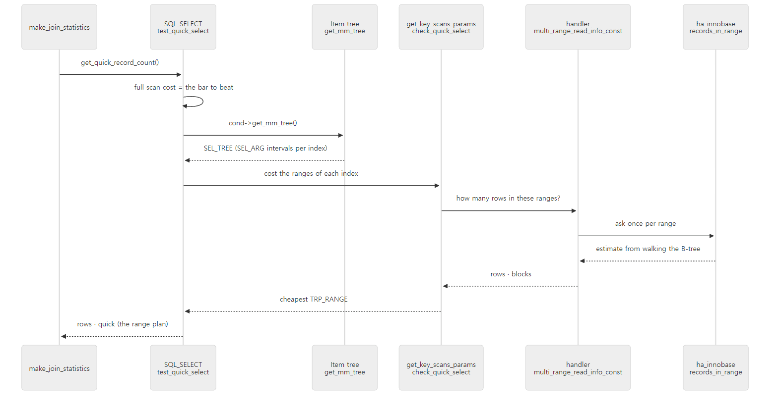 The three on the left are the server layer; the two on the right are the engine side. One EXPLAIN reaches all the way down to the engine's B-tree.
Example 4: how EXPLAIN reaches InnoDB's B-tree
I checked with gdb that it really goes this way. Example ex/u08-gdb-range attaches gdb -p to the running mariadbd, sets break ha_innobase::records_in_range, sends EXPLAIN SELECT * FROM customers WHERE country = 'KR' from another shell, prints the backtrace at the stop (bt) and detaches (detach).
#0  ha_innobase::records_in_range (...) at /usr/src/mariadb/storage/innobase/handler/ha_innodb.cc:14632
#1  0x000055aaf6fcb9e8 in handler::multi_range_read_info_const (...) at /usr/src/mariadb/sql/multi_range_read.cc:247
#2  0x000055aaf6fcf969 in DsMrr_impl::dsmrr_info_const (...) at /usr/src/mariadb/sql/multi_range_read.cc:1791
#3  0x000055aaf7640a8d in ha_innobase::multi_range_read_info_const (...) at /usr/src/mariadb/storage/innobase/handler/ha_innodb.cc:20880
#4  0x000055aaf6b82e90 in check_quick_select (...) at /usr/src/mariadb/sql/opt_range.cc:12543
#5  0x000055aaf6b76a89 in get_key_scans_params (...) at /usr/src/mariadb/sql/opt_range.cc:7996
#6  0x000055aaf6b6966e in SQL_SELECT::test_quick_select (...) at /usr/src/mariadb/sql/opt_range.cc:3036
#7  0x000055aaf6db57f0 in get_quick_record_count (...) at /usr/src/mariadb/sql/sql_select.cc:5525
#8  0x000055aaf6db82f4 in make_join_statistics (...) at /usr/src/mariadb/sql/sql_select.cc:6265
#9  0x000055aaf6dab8a2 in JOIN::optimize_inner (...) at /usr/src/mariadb/sql/sql_select.cc:2779
#10 0x000055aaf6da8bca in JOIN::optimize (...) at /usr/src/mariadb/sql/sql_select.cc:2032
#11 0x000055aaf6db545e in mysql_select (...) at /usr/src/mariadb/sql/sql_select.cc:5447
#12 0x000055aaf6e04c2f in mysql_explain_union (...) at /usr/src/mariadb/sql/sql_select.cc:32912
#13 0x000055aaf6d389d4 in execute_sqlcom_select (...) at /usr/src/mariadb/sql/sql_parse.cc:6205
#14 0x000055aaf6d323a1 in mysql_execute_command (...) at /usr/src/mariadb/sql/sql_parse.cc:4038
#15 0x000055aaf6d3d81e in mysql_parse (...) at /usr/src/mariadb/sql/sql_parse.cc:8005
#16 0x000055aaf6d2c338 in dispatch_command (...) at /usr/src/mariadb/sql/sql_parse.cc:1903
...
(The argument lists were shortened to (...) with sed, and the connection-thread frames below #17 were dropped. Addresses differ from run to run.) Reading from the bottom up: dispatch_command() (Part 5) → mysql_execute_command() → the EXPLAIN branch of execute_sqlcom_select() → mysql_explain_union() → the same mysql_select() → JOIN::optimize() used for execution → make_join_statistics() line 6265 (the get_quick_record_count() call) → the range optimizer → the handler's MRR (Multi-Range Read, the interface for handling many ranges at once) → InnoDB. It matches the order in the diagram. You can also see at #3 that InnoDB overrides the MRR function (ha_innobase::multi_range_read_info_const) and hands it to the server's DS-MRR implementation (DsMrr_impl, sql/multi_range_read.cc), which in turn calls the handler's default function.
Easy to get wrong: EXPLAIN is not free
As the backtrace shows, EXPLAIN also reads the engine's index pages (estimates like this are often called "index dives"). Usually it is a few pages per interval, but an IN (…) with thousands of values means thousands of intervals. That is why eq_range_index_dive_limit exists — once the equality intervals reach that count, it estimates from statistics instead of walking the B-tree. Add the const-table reads from section 3, and EXPLAIN means "does not execute", not "reads nothing".
5. Cost — the new cost model where "1 is one millisecond"
We have used the word "cost" many times now. In this commit, cost is defined in one line at the top of sql/optimizer_defaults.h.
/*
  This file contains costs constants used by the optimizer
  All costs should be based on milliseconds (1 cost = 1 ms)
*/
sql/optimizer_defaults.h lines 21–24
So the 21.23 in Last_query_cost is the optimizer's guess that "this plan will take about 21 milliseconds" (a value computed from constants, not a measured time). This cost model arrived in recent releases — sql/optimizer_costs.h carries a 2022 copyright, and the structure that keeps cost constants per engine lives in that file. I did not confirm from the source which release introduced it.
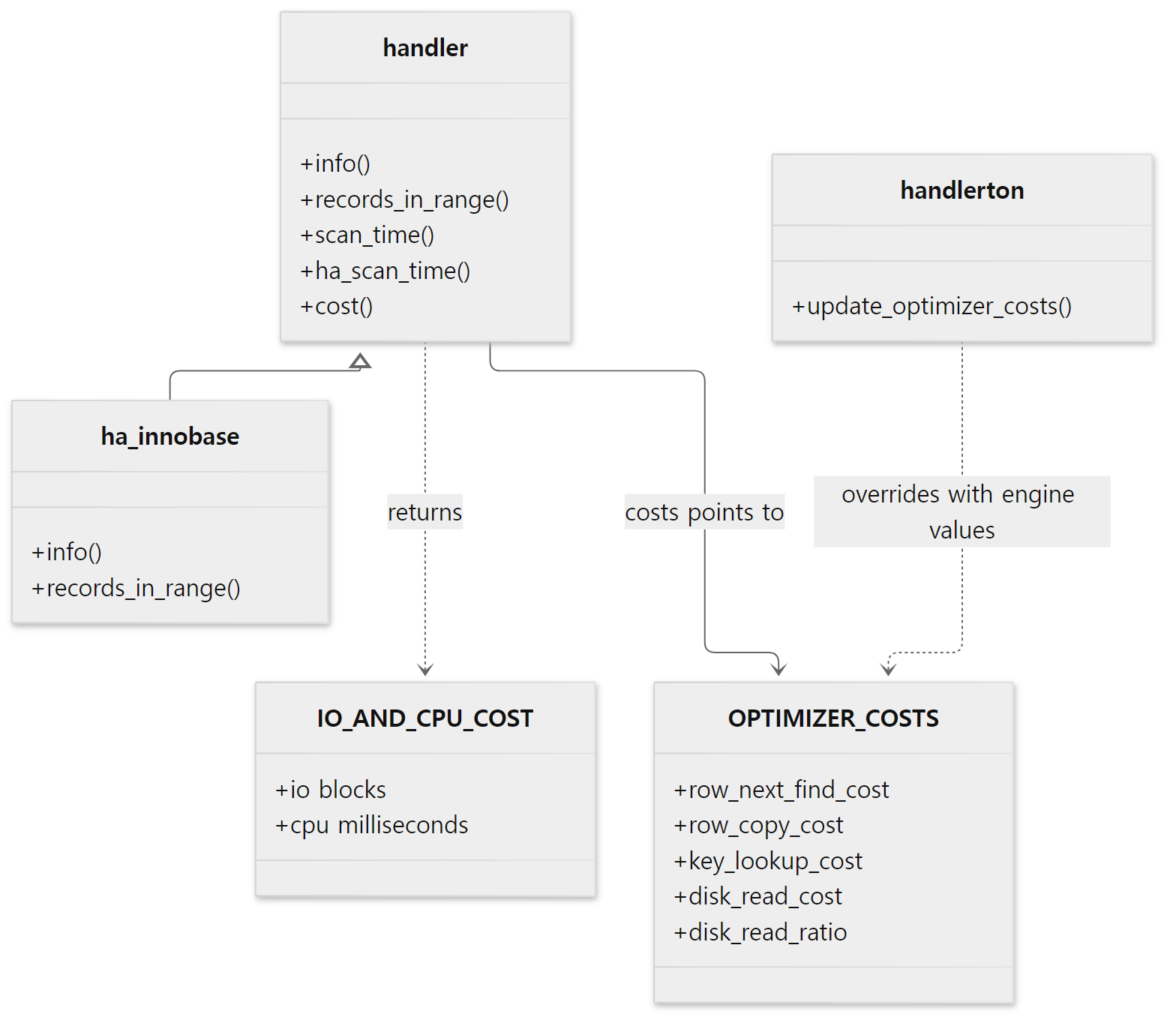 There is one set of cost constants per engine, and the
handler's cost functions compute with those constants.
One set of constants per engine
The cost constants live in a single struct OPTIMIZER_COSTS (sql/optimizer_costs.h lines 32–47) — twelve cost constants (doubles) plus an initialized marker; the constants include finding one key (key_lookup_cost), moving to the next row (row_next_find_cost), copying a row (row_copy_cost) and reading one block (disk_read_cost). The defaults are the DEFAULT_* macros in optimizer_defaults.h (DEFAULT_ROW_NEXT_FIND_COST 0.000045916 and so on), and an engine overrides them with its own values through the update_optimizer_costs function pointer of its handlerton (the one-per-engine struct we saw in Part 3). For InnoDB:
static void innobase_update_optimizer_costs(OPTIMIZER_COSTS *costs)
{
  /*
    The following number was found by check_costs.pl when using 1M rows
    and all rows are cached. See optimizer_costs.txt for details
  */
  costs->row_next_find_cost= 0.00007013;
  costs->row_lookup_cost=    0.00076597;
  costs->key_next_find_cost= 0.00009900;
  costs->key_lookup_cost=    0.00079112;
  costs->row_copy_cost=      0.00006087;
}
storage/innobase/handler/ha_innodb.cc lines 4242–4253
As the comment says, these numbers were measured with a script called check_costs.pl. handler::costs points at them (sql/handler.h line 3486 — "Points to table->share->costs"), and the cost functions use these macros (ROW_NEXT_FIND_COST and friends are aliases for costs->row_next_find_cost and so on).
Cost = disk part + CPU part
A cost function returns an IO_AND_CPU_COST — the number of blocks to read (io) and CPU time (cpu, in milliseconds) — and handler::cost() folds the two into one number.
  inline double io_cost(IO_AND_CPU_COST cost)
  {
    return cost.io * DISK_READ_COST * DISK_READ_RATIO;
  }

  inline double cost(IO_AND_CPU_COST cost)
  {
    return io_cost(cost) + cost.cpu;
  }
The block count is multiplied by "the time to read one block" (DISK_READ_COST) and "the chance that block is not in the cache" (DISK_READ_RATIO). The default disk_read_ratio is 0.02, i.e. it assumes only one read in fifty actually hits the disk (the comment from line 118 of optimizer_defaults.h explains why at length). The cost of a full scan is computed like this.
IO_AND_CPU_COST handler::ha_scan_time(ha_rows rows)
{
  IO_AND_CPU_COST cost;
  bool rc= (table && table->in_use && table->in_use->opt_ctx_replay)
               ? table->in_use->opt_ctx_replay->infuse_ha_scan_time(table, &cost)
               : true;
  if (rc)
  {
    cost= scan_time();
    cost.cpu+= (TABLE_SCAN_SETUP_COST +
                (double) rows * (ROW_NEXT_FIND_COST + ROW_COPY_COST));
  }
  return cost;
}
sql/handler.cc lines 9902–9915
Adding the per-row WHERE check cost (rows * WHERE_COST) to this gives ha_scan_and_compare_time() (sql/handler.h lines 4044–4049), the value test_quick_select() in section 4 uses as its bar.
If the engine does not override scan_time(), the default implementation is used (handler.h lines 4026–4035) — io is the data size divided by IO_SIZE (4096 bytes), and cpu is the page count × INDEX_BLOCK_COPY_COST. InnoDB's ha_innobase::scan_time() is fenced off with #ifdef NOT_USED (ha_innodb.cc line 14798), so it uses the default.
Example 2 (part): computing a full scan cost by hand
Output 0 of Example 2 prints the numbers the optimizer starts from — the row count and data size from information_schema.TABLES, the cost constants from information_schema.OPTIMIZER_COSTS (the default and InnoDB rows), and the cost-related system variables (the SQL is in ex/u08-plan-change/demo.sql).
+------------+------------+-------------+
 TABLE_NAME | TABLE_ROWS | DATA_LENGTH |
+------------+------------+-------------+
 customers  |       1000 |       81920 |
 orders     |      19982 |     1589248 |
+------------+------------+-------------+
+---------+---------------+----------+------------+------------+-----------+-----------------+
 ENGINE  | row_next_find | row_copy | key_lookup | row_lookup | disk_read | disk_read_ratio |
+---------+---------------+----------+------------+------------+-----------+-----------------+
 default |      0.045916 | 0.060866 |   0.435777 |   0.130839 | 10.240000 |        0.020000 |
 InnoDB  |      0.070130 | 0.060870 |   0.791120 |   0.765970 | 10.240000 |        0.020000 |
+---------+---------------+----------+------------+------------+-----------+-----------------+
+------------------------+-----------------------------+--------------------------+
 @@optimizer_where_cost | @@optimizer_scan_setup_cost | @@optimizer_search_depth |
+------------------------+-----------------------------+--------------------------+
               0.032000 |                   10.000000 |                       62 |
+------------------------+-----------------------------+--------------------------+
information_schema.OPTIMIZER_COSTS shows the values multiplied by 1000 (the *1000.0 on lines 10502–10513 of sql/sql_show.cc). The source's 0.00007013 milliseconds shows up as 0.070130 (microseconds). The system variables optimizer_where_cost·optimizer_scan_setup_cost follow the same rule (COST_ADJUST(1000) in sys_vars.cc). Only disk_read_ratio, a ratio, is shown as is.
Now let's reproduce by hand the customers full scan cost of 0.177274 that Example 3 in section 6 will show in the trace (in milliseconds).
| Part | Computation | Value |
|---|---|---|
| Disk | 81920 / 4096 = 20 blocks × 0.01024 × 0.02 | 0.004096 |
| Page copy | 81920 / 16384 = 5 pages × 0.0000356 | 0.000178 |
| Scan setup | optimizer_scan_setup_cost |
0.01 |
| Fetch 1,000 rows | 1000 × (0.00007013 + 0.00006087) | 0.131 |
| WHERE check | 1000 × 0.000032 | 0.032 |
| Total | 0.177274 |
16384 is InnoDB's page size (stats.block_size), and the two row-fetching constants are the InnoDB values above. With nothing but the formulas and constants from the source, the trace's number matches to six decimal places. Once you have a feel for where the optimizer's "cost" comes from, you can also see why 17.88 of the 21.23 in section 1 was c's eq_ref — 17.88 ÷ 19,982 ≈ 0.0009 ms, a key lookup of under a microsecond each, multiplied twenty thousand times.
6. Join order — choose_plan(), greedy_search(), best_access_path()
With N tables there are N! join orders: 6 for 3 tables, 3,628,800 for 10. Picking one of them is the job of choose_plan() (line 10519). With STRAIGHT_JOIN, optimize_straight_join() just computes the cost of the order written in FROM (lines 10577–10580); otherwise greedy_search() searches for an order. If optimizer_search_depth is 0, determine_search_depth() decides (number of tables + 1 when there are 7 or fewer, lines 10852–10869), but the default is not 0 — it is MAX_TABLES + 1 (= 62) (sys_vars.cc lines 3067–3076; Example 2's output also shows 62). MAX_TABLES is 61: the number of bits in a table_map (a 64-bit integer with one bit per table) minus 3 (sql/sql_const.h line 87).
greedy_search and best_extension_by_limited_search
As its name says, greedy_search() fills the order "greedily, one slot at a time". Each round it uses best_extension_by_limited_search() to examine, depth first, up to search_depth slots ahead, commits only the first table of the best extension, and moves on to the next slot. If the number of remaining tables is at most search_depth, a single search finishes the job (if (size_remain <= search_depth) on line 11140). The default of 62 is larger than the number of tables one SELECT can hold (MAX_TABLES), so with default settings it effectively examines every order, apart from pruning.
best_extension_by_limited_search() has two key spots. First it tries putting one candidate table at the end of the plan and adds up the cost.
      /* Compute the cost of the new plan extended with 's' */
      current_record_count= COST_MULT(record_count, position->records_out);
      current_read_time= COST_ADD(read_time, position->read_time);
sql/sql_select.cc lines 12533–12535
record_count (the number of row combinations produced by the tables so far) is multiplied by this table's records_out (rows left in this table after WHERE, per row of the tables before), and the cost is added. Then comes pruning right away.
      /* Expand only partial plans with lower cost than the best QEP so far */
      if (current_read_time + COST_EPS >= join->best_read)
      {
        // ... (DBUG output)
        trace_one_table
          .add("pruned_by_cost", true)
          .add("current_cost", current_read_time)
          .add("best_cost",    join->best_read);

        restore_prev_nj_state(s);
        restore_prev_sj_state(remaining_tables, s, idx);
        continue;
      }
sql/sql_select.cc lines 12561–12577
If this is already more expensive than the best complete plan found so far (best_read), nothing added after it can make it cheaper, so it goes no deeper. Since costs are only ever added, this is a safe call. When optimizer_prune_level (default 2) is 1 or more, a more aggressive heuristic pruning (pruned_by_heuristic, lines 12583–12668) also runs — "drop it if both the row count and the cost are worse than the best at this slot" — and the comment admits it may miss the optimal plan. When a complete plan reached at the bottom is cheaper than the best so far, it is copied into best_positions[].
        if (current_read_time < join->best_read)
        {
          memcpy((uchar*) join->best_positions, (uchar*) join->positions,
                 sizeof(POSITION) * (idx + 1));
          join->join_record_count= partial_join_cardinality;
          join->best_read= current_read_time;
        }
sql/sql_select.cc lines 12759–12765
best_access_path — the cheapest way to put one table in one slot
In "try putting one candidate table at the end of the plan", the function that decides how to read that table is best_access_path() (line 9023). Which methods are available depends on which tables are already in front (the complement of remaining_tables).
- It walks the
KEYUSEs and costs index lookups (ref,eq_ref) (theif (s->keyuse)block on line 9104). A lookup is a candidate only if the value it needs comes from a table in front. Foroafterc,o.customer_id = c.idallowsidx_customer; withoin front, it does not. - Then it costs scans (full scan, the range scan found in section 3, full index scan) (from line 9955).
- It picks the cheaper one. The comparison always has the same shape.
      if (cur_cost + COST_EPS < best.cost)
      {
        trace_access_idx.add("chosen", true);
        best.cost= cur_cost;
sql/sql_select.cc lines 9782–9785
COST_EPS (0.0000001, optimizer_costs.h) is a tiny margin so that when two indexes cost the same, the one seen first wins. According to its comment, the point is to keep test results from wobbling with the path floating-point calculations take.
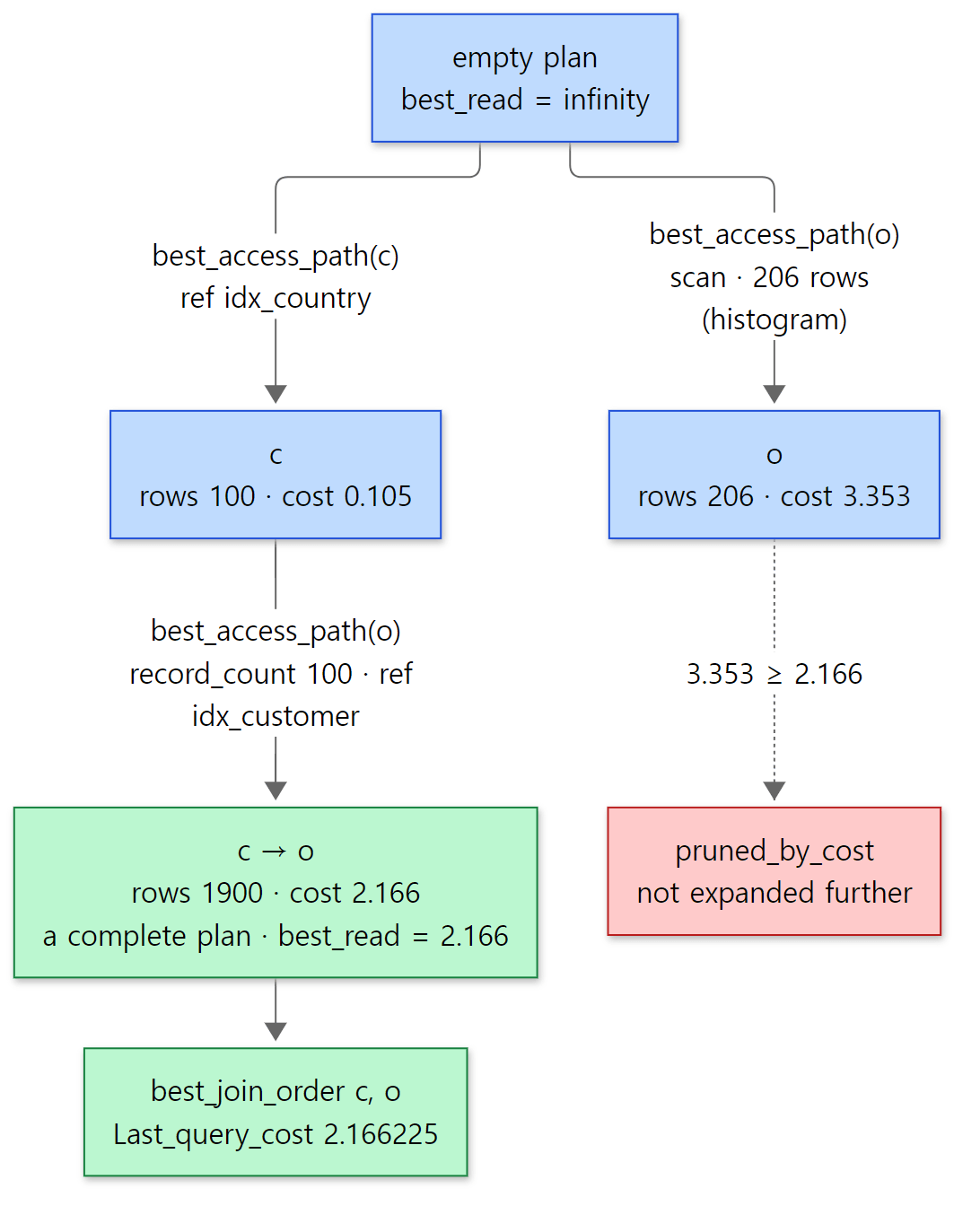 The numbers come from the trace in Example 3 below. The branch starting with
o is cut at the very first slot.
Example 3: watching the search with optimizer_trace
With the optimizer trace (optimizer_trace) turned on, the process above is recorded as JSON. This time orders.customer_id has an index and the status column has a histogram (section 7), and we EXPLAIN the same query as in section 1. The full trace is about 350 lines, so SQL JSON functions pull out just the parts we need.
-- Written for this post (not part of MariaDB's source)
USE shop;
ALTER TABLE orders ADD KEY idx_customer (customer_id);
ANALYZE TABLE orders PERSISTENT FOR COLUMNS (status) INDEXES ();

SET optimizer_trace = 'enabled=on';
-- EXPLAIN runs the optimizer to the end too, so it leaves a trace
EXPLAIN SELECT c.name, o.amount
  FROM customers c JOIN orders o ON o.customer_id = c.id
  WHERE c.country = 'KR' AND o.status = 'cancelled';
-- SHOW STATUS is not traced, so it leaves the trace alone
SHOW SESSION STATUS LIKE 'Last_query_cost';
-- the next SELECT overwrites the trace, so copy it into a variable first
-- (a statement that reads OPTIMIZER_TRACE is itself not traced)
SELECT trace INTO @t FROM information_schema.OPTIMIZER_TRACE;
-- ... (the SELECTs that pull each stage out of @t are omitted)
[Shortened from example ex/u08-optimizer-trace/demo.sql — the extraction SQL is in the example folder]
+------+-------------+-------+------+---------------------+--------------+---------+-----------+------+-----------------------+
 id   | select_type | table | type | possible_keys       | key          | key_len | ref       | rows | Extra                 |
+------+-------------+-------+------+---------------------+--------------+---------+-----------+------+-----------------------+
    1 | SIMPLE      | c     | ref  | PRIMARY,idx_country | idx_country  | 9       | const     | 100  | Using index condition |
    1 | SIMPLE      | o     | ref  | idx_customer        | idx_customer | 4       | shop.c.id | 19   | Using where           |
+------+-------------+-------+------+---------------------+--------------+---------+-----------+------+-----------------------+
+-----------------+----------+
 Variable_name   | Value    |
+-----------------+----------+
 Last_query_cost | 2.166225 |
+-----------------+----------+
With the index in place, the order flipped. It finds the 100 Korean customers through idx_country and, for each customer, looks up orders through idx_customer. Here is what was pulled from the trace, stage by stage (the step label lines are left out).
| transformations                                                             |
 ["equality_propagation","constant_propagation","trivial_condition_removal"] |
 rows_estimation                                                                                                                                                                                                  |
 {"c: table_scan":[{"rows":1000,"cost":0.177274}],"c: range on idx_country":[0.10587704],"o: status histogram":[0.0103],"o: table_scan":[{"rows":20000,"read_cost":2.7129156,"read_and_compare_cost":3.3529156}]} |
(Only the header and the value line of each result are kept, without the table borders.) Item 1 is exactly the names of the three steps of optimize_cond() from section 2. Item 2 is the row estimation from sections 3 and 4.
c's full scan, 0.177274, is the number we reproduced by hand in section 5, and the value test_quick_select() used as its bar. The idx_country range (0.106) was cheaper, so it was accepted. o has no index on status, so there is no range analysis, but the histogram reports that "only 1.03% remains" (0.0103). Items 3 and 4 are this section's search.
+------+--------------+--------+------+--------------+----------+------------+--------+
 tbl  | record_count | access | type | idx          | rows_est | cost       | chosen |
+------+--------------+--------+------+--------------+----------+------------+--------+
 c    |            1 | ref    | NULL | idx_country  |      100 | 0.10508592 | true   |
 c    |            1 | NULL   | scan | NULL         |     NULL |       NULL | false  |
 o    |            1 | scan   | NULL | NULL         |    20000 |  3.3529156 | true   |
 o    |          100 | ref    | NULL | idx_customer |       19 |  2.0611392 | true   |
 o    |          100 | NULL   | scan | NULL         |     NULL |       NULL | false  |
+------+--------------+--------+------+--------------+----------+------------+--------+
+--------+------+---------------+---------------+--------+----------+-----------+------------+
 prefix | tbl  | rows_for_plan | cost_for_plan | pruned | next_tbl | next_rows | next_cost  |
+--------+------+---------------+---------------+--------+----------+-----------+------------+
        | c    |           100 |    0.10508592 | NULL   | o        |      1900 | 2.16622512 |
        | o    |           206 |     3.3529156 | true   | NULL     |      NULL |       NULL |
+--------+------+---------------+---------------+--------+----------+-----------+------------+
+-----------------+----------+------------+
 best_join_order | est_rows | plan_cost  |
+-----------------+----------+------------+
 ["c", "o"]      |    19.57 | 2.16622512 |
+-----------------+----------+------------+
- Each line of table 3 is one candidate
best_access_path()examined.owas evaluated twice. In the first slot (record_count1)refis impossible, soscanis the only candidate; in the slot afterc(record_count100), therefthroughidx_customerappears and wins. That the same table gets a different access method depending on what is in front of it is right there in the table. - Table 4 is the diagram above.
c → ocompleted first at cost 2.166, and the plan starting withowaspruned(pruned_by_cost) because its first slot alone, 3.353, already cost more. - The final 2.16622512 is this query's
Last_query_cost. The example also printsSHOW SESSION STATUS LIKE 'Last_query_cost'right after the EXPLAIN, and it shows 2.166225.
Easy to get wrong: the trace is overwritten by the very next statement
When I first wrote this example, I put lines like SELECT '--- 1. …' AS step; after the EXPLAIN to print stage labels, and read OPTIMIZER_TRACE after them. Every result was NULL. The label-printing SELECT is traced too, so it overwrote the EXPLAIN's trace. The source makes the reason clear: a trace starts fresh for each statement, and at the end only the last one is kept.
void Opt_trace_context::end()
{
  if (current_trace)
    traces.push(current_trace);

  if (!traces.elements())
    return;
  if (traces.elements() > 1)
  {
    Opt_trace_stmt *prev= traces.at(0);
    delete prev;
    traces.del(0);
  }
  current_trace= NULL;
}
sql/opt_trace.cc lines 471–485
What gets traced is SELECT·UPDATE·DELETE·multi-table UPDATE/DELETE·INSERT … SELECT (sql_command_can_be_traced(), lines 110–122). SHOW STATUS and SET are not traced, so they do not overwrite it, and a statement that reads the OPTIMIZER_TRACE table is also excluded (list_has_optimizer_trace_table()). That is why the example copies the trace into @t right after the EXPLAIN and reads only @t afterwards.
7. Statistics change the plan — histograms
In section 1's JSON, o's "filtered": 100 stood out. The optimizer saw status = 'cancelled' as "a condition that filters out nothing". In reality only 1% remains. The ANALYZE statement (unlike EXPLAIN, it actually runs the query and shows the estimate next to the actual value) makes the gap visible (output 5 of Example 1).
ANALYZE SELECT c.name, o.amount
  FROM customers c JOIN orders o ON o.customer_id = c.id
  WHERE c.country = 'KR' AND o.status = 'cancelled';
+------+-------------+-------+--------+---------------------+---------+---------+--------------------+-------+----------+----------+------------+-------------+
 id   | select_type | table | type   | possible_keys       | key     | key_len | ref                | rows  | r_rows   | filtered | r_filtered | Extra       |
+------+-------------+-------+--------+---------------------+---------+---------+--------------------+-------+----------+----------+------------+-------------+
    1 | SIMPLE      | o     | ALL    | NULL                | NULL    | NULL    | NULL               | 19982 | 20000.00 |   100.00 |       1.03 | Using where |
    1 | SIMPLE      | c     | eq_ref | PRIMARY,idx_country | PRIMARY | 4       | shop.o.customer_id | 1     | 1.00     |    10.00 |       9.71 | Using where |
+------+-------------+-------+--------+---------------------+---------+---------+--------------------+-------+----------+----------+------------+-------------+
The columns starting with r_ are the actual values. o's filtered of 100 against an r_filtered of 1.03 — the estimate was off by a factor of 100. c's filtered of 10 was right: country has an index, so range analysis reported "100 out of 1,000". status has neither an index nor statistics, so the optimizer has no way of knowing.
What tells it is Engine-Independent Table Statistics. Collected with ANALYZE TABLE … PERSISTENT FOR …, the server scans the table and stores them in mysql.table_stats·mysql.column_stats·mysql.index_stats (collect_statistics_for_table() in sql/sql_statistics.cc, line 2753), keeping a column's value distribution as a histogram. The default histogram_type is JSON_HB (a height-balanced histogram stored as JSON), and the reading side is Histogram_json_hb in sql/opt_histogram_json.cc — point_selectivity() (line 821) computes the selectivity of a single value and range_selectivity() (line 888) that of an interval.
Whether the optimizer uses these statistics is decided by two variables. use_stat_tables (default PREFERABLY_FOR_QUERIES — sys_vars.cc lines 7372–7376) means "if statistics tables exist, prefer them over engine statistics" (check_eits_preferred(), sql/sql_statistics.h lines 118–123), and optimizer_use_condition_selectivity (default 4) sets how far selectivity is taken into account. In the source there are three thresholds.
| Value | What it does | Where |
|---|---|---|
| 2 or more | calls calculate_cond_selectivity_for_table() |
sql_select.cc line 6294 |
| 3 or more | builds a pseudo index for each non-indexed column and runs section 4's range analysis (get_mm_tree()) on it as is |
opt_range.cc line 3738 |
| 4 or more | reads that column's histogram to get the selectivity of the interval | sql_statistics.cc line 3264 |
The trick used from 3 upwards is a nice one. Even a column with no index is fed into the range optimizer "as if it had an index" to get intervals, and those intervals are then asked of the histogram instead of a B-tree (the comment on lines 3773–3785). The same component is used twice.
Example 2: the same query, EXPLAINed five times
This time we drop the country condition and look only for "cancelled orders and their customer names". We added an index and statistics one at a time and EXPLAINed after each (the same query at every step; only the plan table and Last_query_cost are shown).
--- 1. no index on orders.customer_id
    1 | SIMPLE      | o     | ALL    | NULL          | NULL    | NULL    | NULL               | 19982 | Using where |
    1 | SIMPLE      | c     | eq_ref | PRIMARY       | PRIMARY | 4       | shop.o.customer_id | 1     |             |
 Last_query_cost | 21.226778 |
--- 2. add an index
    1 | SIMPLE      | c     | ALL  | PRIMARY       | NULL         | NULL    | NULL      | 1000 |             |
    1 | SIMPLE      | o     | ref  | idx_customer  | idx_customer | 4       | shop.c.id | 19   | Using where |
 Last_query_cost | 19.970285 |
--- 3. collect a histogram on orders.status
 orders     | status      | JSON_HB   | [{"start": "cancelled", "size": 0.0103, "ndv": 1}, {"start": "done", "end": "done", "size": 0.9897, "ndv": 1}] |
    1 | SIMPLE      | o     | ALL    | idx_customer  | NULL    | NULL    | NULL               | 20000 |     1.03 | Using where |
    1 | SIMPLE      | c     | eq_ref | PRIMARY       | PRIMARY | 4       | shop.o.customer_id | 1     |   100.00 |             |
 Last_query_cost | 3.541266 |
--- 4. same statistics, histogram ignored
    1 | SIMPLE      | c     | ALL  | PRIMARY       | NULL         | NULL    | NULL      | 1000 |   100.00 |             |
    1 | SIMPLE      | o     | ref  | idx_customer  | idx_customer | 4       | shop.c.id | 19   |   100.00 | Using where |
 Last_query_cost | 19.970285 |
--- 5. STRAIGHT_JOIN keeps the FROM order
    1 | SIMPLE      | c     | ALL  | PRIMARY       | NULL         | NULL    | NULL      | 1000 |             |
    1 | SIMPLE      | o     | ref  | idx_customer  | idx_customer | 4       | shop.c.id | 19   | Using where |
 Last_query_cost | 19.970285 |
[Only the data lines from the output of example ex/u08-plan-change, without table headers and borders. Steps 3 and 4 use EXPLAIN EXTENDED to show the filtered column]
- Without the index: scan
oand look upctwenty thousand times (21.23). - With the index: scanning
cand looking up each customer's orders throughidx_customer(19.97) became slightly cheaper, so the order flipped. With no country condition this time,cisALL. - With the histogram:
ocame back to the front and the cost dropped to 3.54. Thefilteredof 1.03 is why. The cost of scanningo(3.35) is almost unchanged, but the optimizer now knows that 206 rows, not twenty thousand, pass WHERE and move on to the next table, so the number ofclookups also drops to 206. Section 6'scurrent_record_count= COST_MULT(record_count, position->records_out)is exactly that multiplication. You can also seerowschange from 19982 to 20000:ANALYZE TABLE … PERSISTENTleft the exact row count inmysql.table_stats, and, as theuse_stat_tablesdefault says, it was preferred over the engine's estimate. - Lowering
optimizer_use_condition_selectivityto 1 with the same statistics: the histogram exists but is not used (below threshold 2 in the table above), so the plan goes back to step 2. STRAIGHT_JOIN: forcing the FROM order (cfirst) makesoptimize_straight_join()only compute the cost. The same plan as step 2 comes out at the same cost.
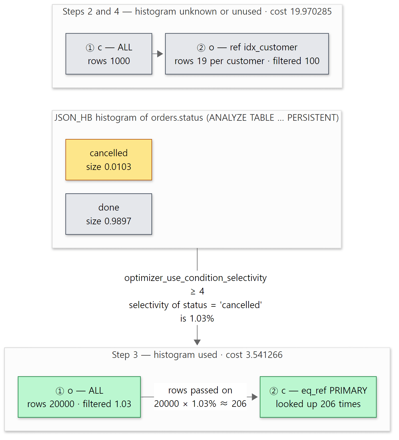 Once one filtered value changed, the order and the cost changed with it. The numbers are Example 2's actual output (ex/u08-plan-change).
Easy to get wrong: there are two kinds of ANALYZE TABLE
The ANALYZE TABLE customers, orders; at the end of the example's setup.sql refreshes only the engine statistics (InnoDB recalculates its own statistics). No histogram is created. Only with PERSISTENT FOR, as in step 3's ANALYZE TABLE orders PERSISTENT FOR COLUMNS (status) INDEXES (), does the server scan the table and write statistics and a histogram to mysql.column_stats. The Engine-independent statistics collected line in the output is the sign. The comment on lines 22–31 of sql/sql_statistics.h says it plainly: with use_stat_tables set to a …_FOR_QUERIES value, a plain ANALYZE TABLE does not collect these statistics. Because they share a name, it is easy to run one and believe you ran both.
8. Where EXPLAIN and optimizer_trace come from
EXPLAIN — a separate copy of the plan
build_explain() at the end of JOIN::optimize() makes the data EXPLAIN will print separately.
  MEM_ROOT *old_mem_root= thd->mem_root;
  // ...
  thd->mem_root= thd->lex->explain->mem_root;
  bool res= save_explain_data(thd->lex->explain, false /* can overwrite */,
                        need_tmp,
                        !skip_sort_order && !no_order && (order || group_list),
                        select_distinct);
  thd->mem_root= old_mem_root;
  DBUG_ASSERT(thd->free_list == old_free_list); // no Items were created
sql/sql_select.cc lines 1966–1974
It temporarily swaps thd->mem_root for the memory area of Explain_query and calls save_explain_data(). As the comment says, no Item may go into this data. The JOIN and its Item trees are cleaned up when execution ends, but the EXPLAIN data must outlive them — when another connection looks at a running query's plan with SHOW EXPLAIN FOR <connection id>, or when ANALYZE prints the plan after execution has finished. So it is copied out as text and numbers (MEM_ROOT is the server's memory pool we saw in Part 2).
The data is a tree of Explain_query → Explain_select (one SELECT) → Explain_table_access (one line of EXPLAIN) (sql/sql_explain.h). Explain_table_access has fields such as type, rows, filtered and cost, and each output format has its own function — tabular is Explain_table_access::print_explain() (sql_explain.cc line 1533), JSON is print_explain_json() (line 2001).
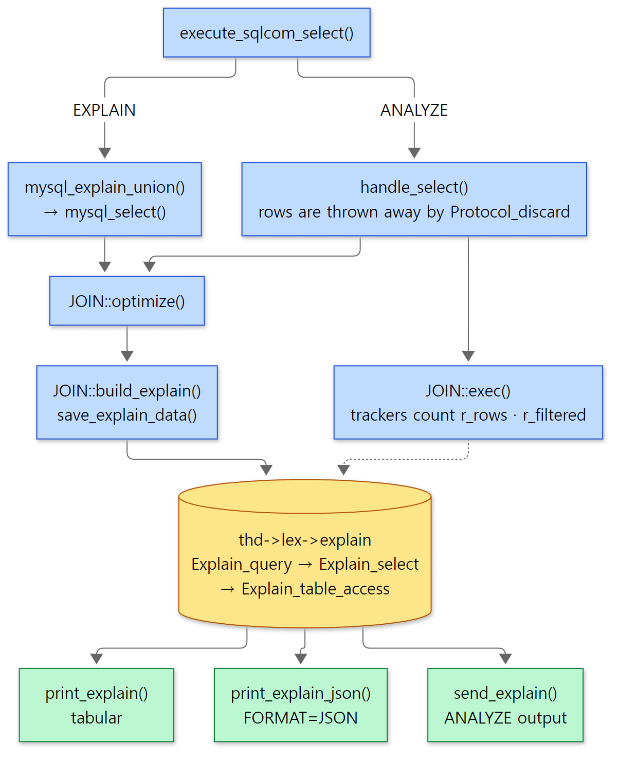 The yellow cylinder is the separately copied EXPLAIN data. EXPLAIN and ANALYZE use the same data; only ANALYZE runs the query and fills in the actual values.
The two paths split in execute_sqlcom_select(). EXPLAIN only optimizes, through mysql_explain_union(), then calls print_explain_json() if lex->explain_json is set and print_explain() otherwise (lines 6189–6222). ANALYZE really runs the query but does not send the result rows to the client.
      if (lex->analyze_stmt)
      {
        // ... (the usual case, with no object intercepting the result)
          result= new (thd->mem_root) select_send_analyze(thd);
          save_protocol= thd->protocol;
          thd->protocol= new Protocol_discard(thd);
        // ...
      res= handle_select(thd, lex, result, 0);
      // ... (restores the protocol)
        if (!res)
        {
          bool extended= thd->lex->describe & DESCRIBE_EXTENDED;
          res= thd->lex->explain->send_explain(thd, extended);
        }
sql/sql_parse.cc lines 6248–6281
It swaps in Protocol_discard (a Protocol that takes rows and throws them away), runs the query with the ordinary handle_select(), and then sends the same EXPLAIN data with send_explain(). During execution, the trackers in Explain_table_access (Table_access_tracker tracker and others) count the rows actually read, and those become r_rows·r_filtered. Everything is real except sending the result rows (Part 5's Protocol).
optimizer_trace — JSON writers embedded all over the optimizer
The trace is not a separate stage; it is embedded throughout the optimizer code. optimize_cond()'s Json_writer_object equal_prop_wrapper(thd), test_quick_select()'s Json_writer_object table_rec(thd, "table_scan") and best_extension_by_limited_search()'s trace_one_table.add("pruned_by_cost", true) that we saw above are all trace records. When tracing is off these objects write nothing, and expensive records are skipped altogether with if (unlikely(thd->trace_started())).
The place that opens and closes the trace for each statement is Opt_trace_start ots(thd); in mysql_execute_command() (sql_parse.cc line 3735). A comment in sql/opt_trace.h lines 80–101 explains that Opt_trace_start::init() is inlined so that, when tracing is off, it checks a single flag and returns. The destructor closes the JSON and calls the Opt_trace_context::end() we saw in section 6. A trace larger than optimizer_trace_max_mem_size (1 MB by default — sys_vars.cc lines 3152–3156) is truncated.
What this post leaves out
- Subquery optimization — semi-join conversion
convert_join_subqueries_to_semijoins()(sql/opt_subselect.ccline 1181), choosing a semi-join strategyoptimize_semijoin_nests()(line 2548),IN→EXISTS, materialization - Merging derived tables and views, and pushing conditions into them —
handle_derived(…, DT_MERGE),pushdown_cond_for_derived()(sql_select.cclines 2567–2605) - Index merge (
index_merge) and ROR intersection —get_best_ror_intersect()(opt_range.ccline 7462); loose index scanget_best_group_min_max()(line 14748) - Plans that finish
ORDER BY … LIMITwithout sorting —join_limit_shortcut_finalize_plan()(sql_select.ccline 12189),test_if_skip_sort_order() - Rowid filters —
JOIN::make_range_rowid_filters()(line 2091) - Table elimination (dropping unused outer-join tables) —
eliminate_tables()(sql/opt_table_elimination.ccline 739) - Partition pruning —
prune_partitions()(opt_range.ccline 4188) - Join buffers and hash joins (
hash_ALLand friends) — Part 9 - Optimizer hints —
sql/opt_hints.cc,sql/opt_hints_parser.cc - Recording and replaying the optimizer context (
optimizer_record_context) —sql/opt_context_store_replay.cc - Two-phase optimization (split materialization) —
check_two_phase_optimization(),JOIN::optimize_stage2_and_finish()(line 2056)
Summary
| Concept | One-line summary |
|---|---|
JOIN::optimize() |
Runs once. build_explain() after optimize_inner(), and the chosen cost goes to Last_query_cost |
optimize_cond() |
Equality propagation → constant propagation → trivial condition removal. Always false means Impossible WHERE |
simplify_joins() |
If WHERE rejects NULLs from the right-hand table, a LEFT JOIN becomes a JOIN |
make_join_statistics() |
Row counts from handler::info(), const tables read on the spot, ranges and selectivity, then choose_plan() |
| Const table | Read during optimization when a unique key is bound to constants. Handler_read_key goes up on EXPLAIN alone |
test_quick_select() |
With the full scan cost as the bar, costs the intervals built by get_mm_tree() for each index |
SEL_TREE/SEL_ARG |
WHERE turned into intervals on indexes. AND is tree_and(), OR is tree_or() |
records_in_range() |
The engine estimates the rows in an interval. InnoDB walks down the B-tree to count |
| Cost model | 1 = one millisecond. Blocks × disk read × cache-miss ratio + CPU. Constants per engine |
greedy_search() |
Looks search_depth slots ahead and commits one slot at a time. Default 62, so effectively exhaustive |
best_extension_by_limited_search() |
Multiplies rows, adds costs, and cuts a branch once it costs more than the best |
best_access_path() |
Depending on the tables in front, the cheapest of ref/eq_ref, range and full scan |
| Histogram | Collected with ANALYZE TABLE … PERSISTENT FOR. When filtered changes, the join order changes |
| EXPLAIN data | An Explain_* tree copied out without Items. ANALYZE runs the query and fills in r_* |
| optimizer_trace | Json_writers throughout the optimizer. Written fresh for each statement; only the last one is kept |
What's next
The plan is settled. The JOIN_TAB array has been built in best_positions[] order, and each table's conditions and read function are decided. Now JOIN::exec() runs that array as nested loops and calls the handler. How Example 1's plan, "scan o and look up c with eq_ref for each row", turns into real calls to rr_sequential() and join_read_key(), and then ha_innobase::rnd_next()·index_read(), is in Part 9: Execution and the Handler API — How the Nested-Loop Join Calls the Engine. That is also where we see where Handler_read_key, which this post only saw as a number, goes up by one.
In earlier series we met code that "picks one out of several candidates" twice. Tomcat Part 7's Mapper picks by a fixed order of rules set by the Servlet spec (exact → longest prefix → extension → default), and Spring Part 22's RequestMappingHandlerMapping gathers candidates and picks "the most specific" with a comparator. The optimizer does the same job with estimated numbers. That is why the same SQL can get a different answer when indexes and statistics change, as Example 2 shows.
On the application side, you usually need this post when you run into a "slow query". Take the SQL sent by Spring Part 18's JdbcTemplate or Spring Part 19's JPA, put it into EXPLAIN·ANALYZE as is, and if filtered and r_filtered differ a lot, suspect a missing histogram first; if the index you expected is not even in possible_keys, suspect the shape of the condition from section 2 (a LEFT JOIN, a column wrapped in a function).
- Part 2: The Big Picture — the Server Layer, Storage Engines, and the Life of One Query
- Part 6: The Parser — How an SQL Statement Becomes LEX and Item Trees
- Part 7: Preparation — Checking Privileges, Opening Tables, Resolving Names
- Part 10: InnoDB Part 1 — Pages, the Buffer Pool and B-trees — what the B-tree that
records_in_range()walks down looks like